Gaussian Processes for Regression and Classification
With the latest HeuristicLab version 3.3.8 we released an implementation of Gaussian process models for regression analysis. Our purely managed C# implementation is mainly based on the MATLAB implementation by Rasmussen and Nickisch accompanying the book "Gaussian Processes for Machine Learning" by Rasmussen and Williams (available online).
If you want to try Gaussian process regression in HeuristicLab, simply open the preconfigured sample. You can also import a CSV file with your own data.
The Gaussian process model can be viewed as a Bayesian prior distribution over functions and is related to Bayesian linear regression.
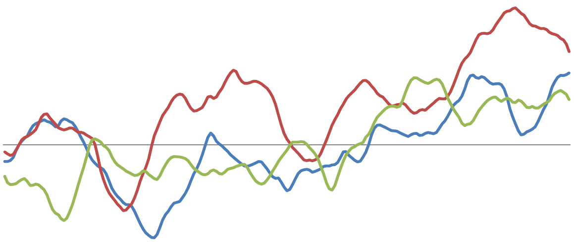
Samples from two different one-dimensional Gaussian processes:
Similarily to other models, such as the SVM, the GP model also uses the 'kernel-trick' to handle high-dimensional non-linear projections to feature space efficiently.
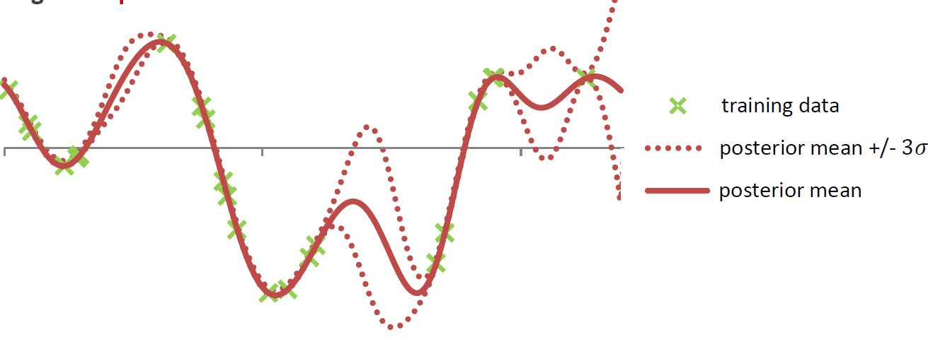
'Fitting' the model means to calculate the posterior Gaussian process distribution by conditioning the GP prior distribution on the observed data points in the training set. This leads to a posterior distribution in which functions that go through the observed training points are more likely. From the posterior GP distribution it is easily possible to calculate the posterior predictive distribution. So, instead of a simple point prediction for each test point it is possible to use the mean of the predictve distribution and calculate confidence intervals for the prediction at each test point.
The model is non-parametric and is fully specified via a mean function and a covariance function. The mean and covariance function often have hyper-parameters that have to be optimized to fit the model to a given training data set. For more information check out the book.
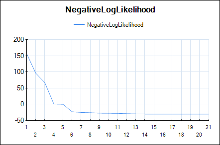
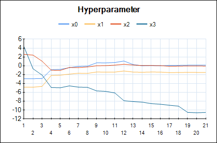
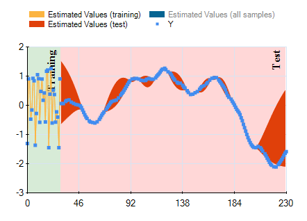
In HeuristicLab hyper-parameters of the mean and covariance functions are optimized w.r.t. the likelihood function (type-II ML) using the gradient-based BFGS algorithm. In the GUI you can observe the development of the likelihood and the values of the hyper-parameters over BFGS iterations. The output of the final Gaussian process model can also be visualized using a line chart that shows the mean prediction and the 95% confidence intervals.
Line chart of the negative log-likelihood:
Line chart of the optimized hyper-parameters:
Output of the model (mean and confidence interval):
We observed Gaussian process models often produce very accurate predictions, especially for low-dimensional data sets with up to 5000 training points. For larger data sets the computational effort becomes prohibitive (we have not yet implemented sparse approximations).
Math notation for symbolic models
In February I have a little more time available that I can spend on HeuristicLab development. So I implemented a new view that shows genetic programming solutions for symbolic data analysis problems in conventional math notation. This has been on our wishlist for a long time, however, up to now we didn't see a good way of implementing this. The implementation is not ideal because it relies on the MathJax library (Javascript) to display the models in a webbrowser control. Using the daily build of the trunk version you can try this new feature. I hope you find it useful.
Financial Analysis with HeuristicLab
One application that I've been interested in lately is financial analysis.
Recently I've looked at interest rate swaps in more detail. Interest rate swaps are an important financial instrument for controlling risk, but are also used for speculative purposes. Using the genetic programming capabilities of HeuristicLab it is relatively easy to generate a regression model to estimate the interest rate swap yield. The result for the European 10-year interest rate swap (monthly data) in the time span from April 1991 until August 2011 can be seen in the next figure.
In the last section from index 582 onwards (July 2007 - August 2011) the output of the model (red line) deviates very strongly from the actually observed values.
To get a better idea of the underlying relations found by GP it is interesting to study variable impacts. The most important variables for the 10-year European interest rate swap yield found through the genetic programming runs are:
| Most relevant variables | Hold out set |
|---|---|
| US M1, US Mortgage Market Index | March 1991 - April 1995 |
| Eurozone Employment qq, US M1, US Corporate Profits | April 1995 - May 1999 |
| US Corporate Profits, Eurozone Employment qq, US U Michigan Expectations Prelim. | May 1999 - June 2003 |
| US Corporate Profits, Eurozone Employment qq | June 2003 - July 2007 |
| US Existing Home Sales | July 2007 - August 2008 |
Interestingly the most important variables differ for different time spans. Only the corporate profits and the number of employed persons in the Euro zone are detected as relevant over a larger time span.
The following table shows the variable impact calculation results for the first fold in greater detail. It can be clearly seen that money supply M1 in the US and the US mortgage market index are used repeatedly in all models. This is a strong indicator that there is a strong correlation of these variables and the interest rate swap yield for the time span from April 1995 until August 2011 which was used as training set for these models. As can be seen in the previous chart the output on the hold out set (March 1991 - April 1995) is relatively accurate.

New Feature for System Identification: Model Response View
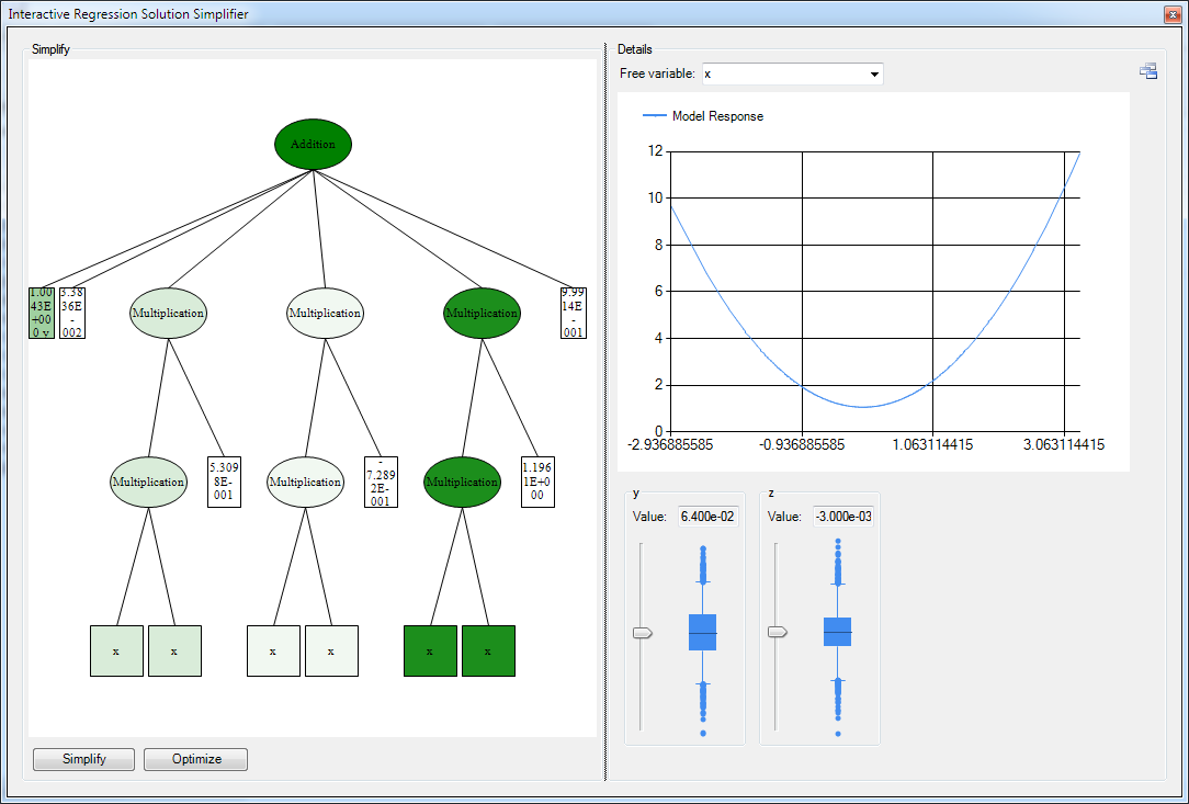
Last week I implemented a new view for symbolic regression models that makes it possible to analyse the impact of a given input variable on the output of the model in more detail. I'm already looking forward to apply it to real world scenarios.
The development efforts for this feature are tracked in ticket #1621

 rss
rss

