
 rss
rss
Gaussian Processes for Regression and Classification
With the latest HeuristicLab version 3.3.8 we released an implementation of Gaussian process models for regression analysis. Our purely managed C# implementation is mainly based on the MATLAB implementation by Rasmussen and Nickisch accompanying the book "Gaussian Processes for Machine Learning" by Rasmussen and Williams (available online).
If you want to try Gaussian process regression in HeuristicLab, simply open the preconfigured sample. You can also import a CSV file with your own data.
The Gaussian process model can be viewed as a Bayesian prior distribution over functions and is related to Bayesian linear regression.
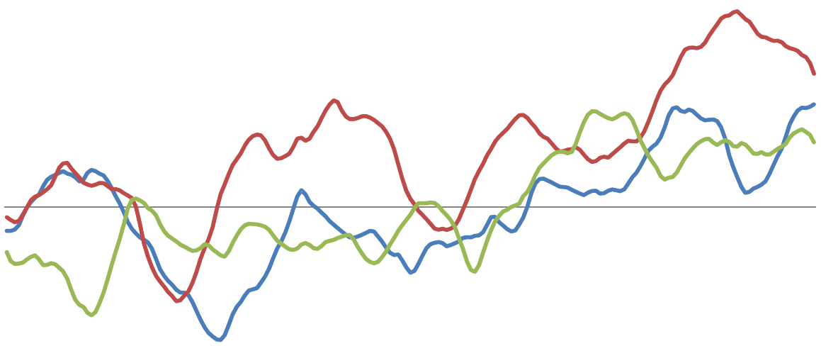
Samples from two different one-dimensional Gaussian processes:


Similarily to other models, such as the SVM, the GP model also uses the 'kernel-trick' to handle high-dimensional non-linear projections to feature space efficiently.
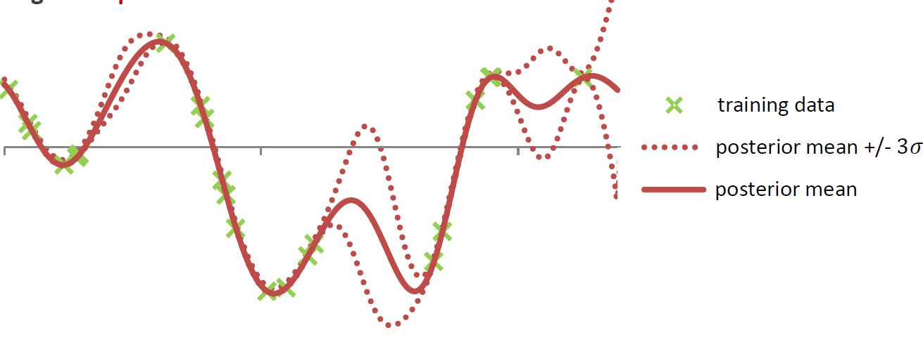
'Fitting' the model means to calculate the posterior Gaussian process distribution by conditioning the GP prior distribution on the observed data points in the training set. This leads to a posterior distribution in which functions that go through the observed training points are more likely. From the posterior GP distribution it is easily possible to calculate the posterior predictive distribution. So, instead of a simple point prediction for each test point it is possible to use the mean of the predictve distribution and calculate confidence intervals for the prediction at each test point.

The model is non-parametric and is fully specified via a mean function and a covariance function. The mean and covariance function often have hyper-parameters that have to be optimized to fit the model to a given training data set. For more information check out the book.
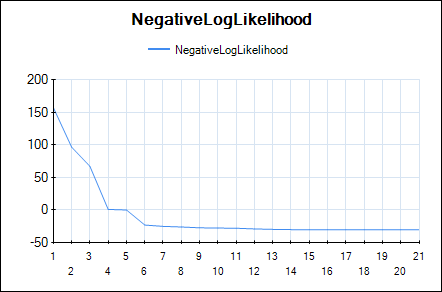
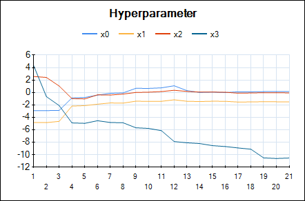
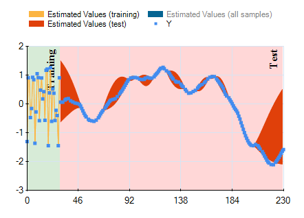
In HeuristicLab hyper-parameters of the mean and covariance functions are optimized w.r.t. the likelihood function (type-II ML) using the gradient-based BFGS algorithm. In the GUI you can observe the development of the likelihood and the values of the hyper-parameters over BFGS iterations. The output of the final Gaussian process model can also be visualized using a line chart that shows the mean prediction and the 95% confidence intervals.
Line chart of the negative log-likelihood:

Line chart of the optimized hyper-parameters:

Output of the model (mean and confidence interval):

We observed Gaussian process models often produce very accurate predictions, especially for low-dimensional data sets with up to 5000 training points. For larger data sets the computational effort becomes prohibitive (we have not yet implemented sparse approximations).
Attachments (6)
- GP samples I.png (38.4 KB) - added by gkronber 11 years ago.
- GP samples II.png (45.2 KB) - added by gkronber 11 years ago.
- GP learning.png (43.3 KB) - added by gkronber 11 years ago.
- GP likelihood.png (5.9 KB) - added by gkronber 11 years ago.
- GP hyperparams.png (11.4 KB) - added by gkronber 11 years ago.
- GP model.png (16.1 KB) - added by gkronber 11 years ago.
Download all attachments as: .zip
Comments
No comments.